水波#

Let’s review this demo script in detail. Afterwards, you should be able to script your own tree.

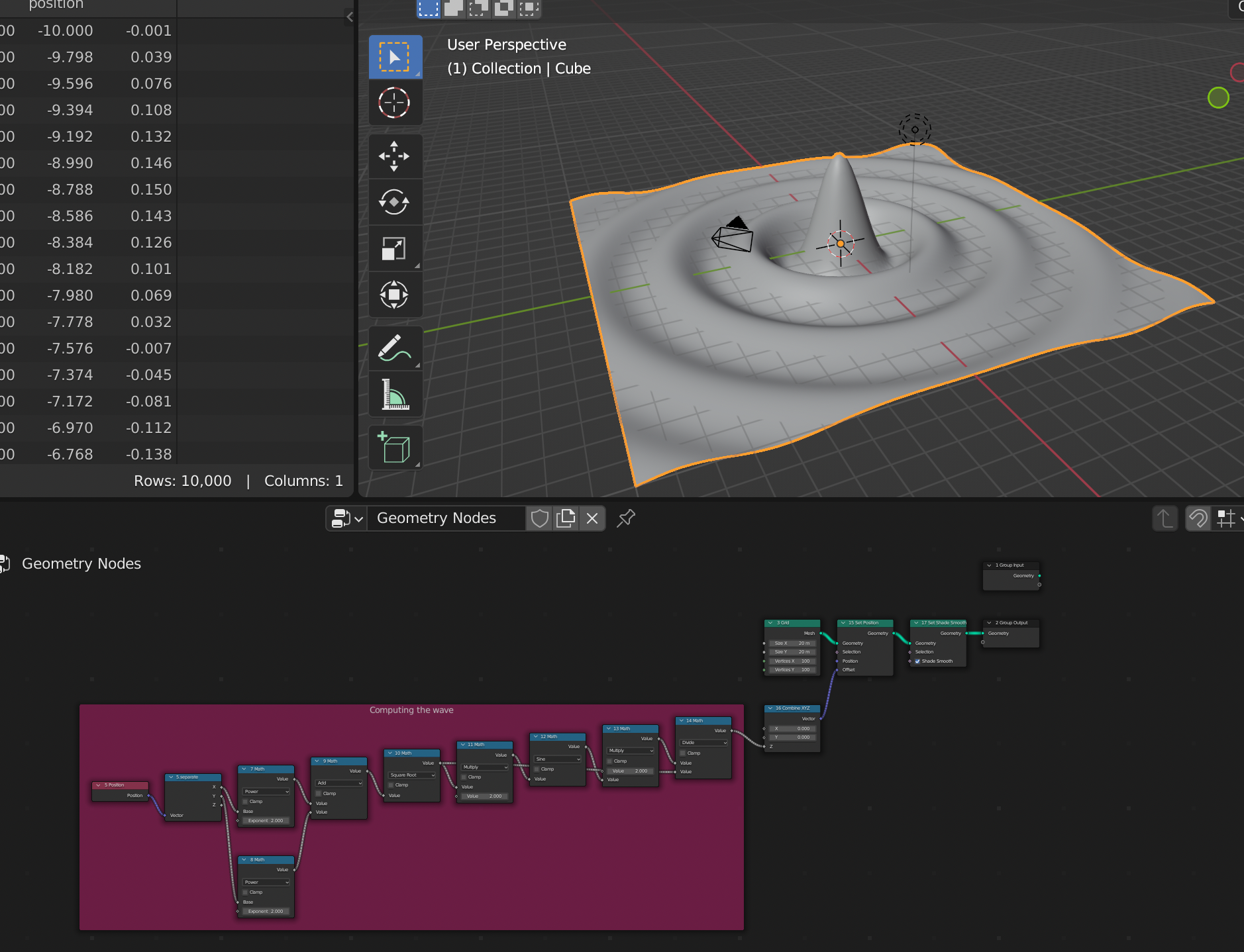
The script creates a surface from a grid by computing \(z = sin(d)/d\) where \(d=\sqrt{x^2 + y^2}\) is the distance of the vertex to the center.

import geonodes as gn

with gn.Tree("Geometry Nodes") as tree:

    # Let's document our parameters
    count  = 100  # Grid resolution
    size   = 20   # Size
    omega  = 2.   # Period
    height = 2.   # Height of the surface
    
    # The base (x, y) grid
    grid = gn.Mesh.Grid(vertices_x=count, vertices_y=count, size_x=size, size_y=size)
    
    # We compute z
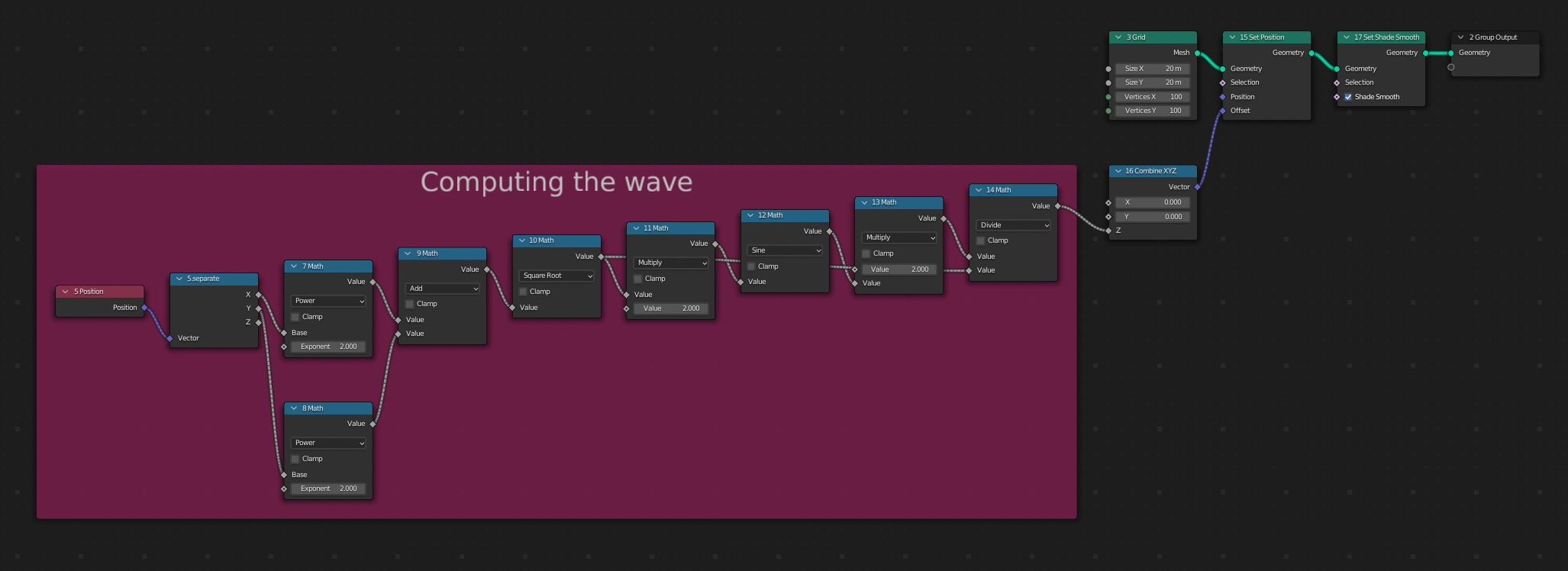
    with tree.layout("Computing the wave", color="dark_rose"):
        distance = gn.sqrt(grid.verts.position.x**2 + grid.verts.position.y**2)
        z = height * gn.sin(distance*omega)/distance
        
    # Let's change the z coordinate of our vertices
    grid.verts.position += (0, 0, z)
    
    # We are done: plugging the deformed grid as the modified geometry
    tree.output_geometry = grid.set_shade_smooth()
                   

The generated nodes and the result of the Geometry nodes modifier is given below:

Description#

Import#

import geonodes as gn

Be sure to have properly installed the geonodes module as described in the Installation section.

gn is the proposed alias to use as geonodes naming space.

Tree creation#

A Tree instance can be created with

tree = Tree(tree_name)
...
tree.close()

But it is recommanded to use with syntax to ensure that the tree will be properly closed. The closing performs final mandatory treatments.

with gn.Tree("Geometry Nodes") as tree:
    ...

The tree_name is the name of a geometry nodes modifier. If it doesn’t exist, it will be created.

Warning when calling tree(tree_name), all the nodes and links are erased. Be sure not to open a tree with an existing valuable tree you don’t want to loose.

The tree can be created with the argument group=True when the generated tree is not to be used as a modifier:

with gn.Tree("Custom function", group=True):
   ...

With the default option group=False, first sockets (input and output) are Geometry.

Within the scope of a Tree creation / closure, all nodes are created within this tree without the need to make explicit reference to this tree.

In the following example, the grid mesh is created in tree without making any explicit reference to it.

with gn.Tree("Geometry Nodes') as tree:

    grid = gn.Mesh.Grid(vertices_x=count, vertices_y=count, size_x=size, size_y=size)

Fore more details, see class Tree reference

Variables#

You can use standard Python variables:

    count  = 100  # Grid resolution
    size   = 20   # Size
    omega  = 2.   # Period
    height = 2.   # Height of the surface

The variables can be used for standard python computing:

# We need an angle of 30 degrees
angle = math.pi / 6

The variables can also be used as default values of node sockets:

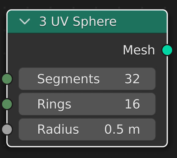
# Let's create an UV sphere of radius 0.5
r = 0.5
sphere = gn.Mesh.UVSphere(radius=r)

In the created node, the input socket radius is initialized with 0.5:

Geonodes types#

In this example, the variables are initialized in the script. They are pure Python variables. To change them, one needs to modify the script and to rerun it.

When creating a tree, we often need to change settings to see the effect on the geometry. This can be achieved by initializing a geonodes type rather than a python type.

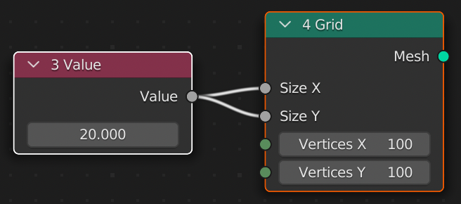
In the following script, we slightly modify our code by initializing size as a geonodes type. It is not anymore a Python float but a geonodes Float i.e. the output socket of a Geometry Node (in that case, the output socket of the input node ‘Value’):

    count  = 100
    size   = gn.Float(20.)
    
    grid = gn.Mesh.Grid(vertices_x=count, vertices_y=count, size_x=size, size_y=size)

The resulting tree is the following. The two Vertices input sockets are initialized with the same value. The two Size sockets are linked to the output socket of a ‘Value’ node. One can change the value of the node to see the result on the output geometry.

Note: remember that the nodes are deleted a each run of the script. Hence, if you change the value in a node, the change will be lost next time you will run the script. To avoid that, either your put the value you want in the script or your read the next section.

Group inputs#

Rather that creating an input Node to initialize your data, you can use a group socket, i.e. a Group input socket. All data socket classes expose the constructor method Input.

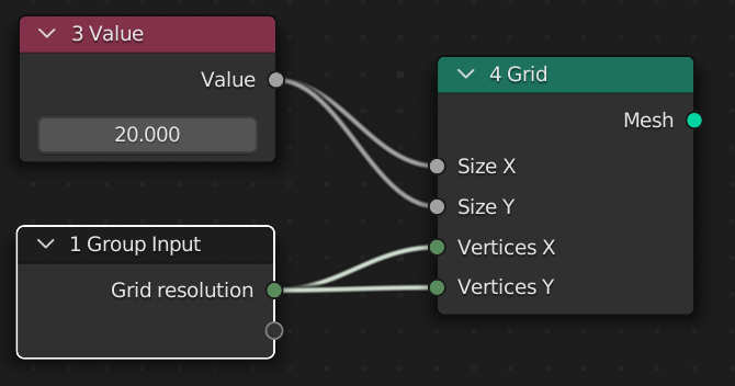
Let’s modify our script. This time, we initialize count as being a Group input socket.

Note: an input socket of the modifier is an output socket of the node ‘Group Input’.

    count  = gn.Integer.Input(100, "Grid resolution")
    size   = gn.Float(20.)
    
    grid = gn.Mesh.Grid(vertices_x=count, vertices_y=count, size_x=size, size_y=size)

In the resulting tree, the node ‘Grid’ is now fed by one node and a user parameter named ‘Grid resolution’:

Geometry creation#

In our demo, the initial grid is created with the following line:

    grid = gn.Mesh.Grid(vertices_x=count, vertices_y=count, size_x=size, size_y=size)

Geometry creation is done through the nodes located in the Blender add menus Mesh Primitives and Curve Primitives.

In geonodes, these nodes are implemented as constructors (class or static methods) of Mesh of Curve classes.

Layouts#

Layouts are ways to make the trees clearer. Creating a layout is done in the context of with syntax: any new node created in the scope of a with is included in the layout:

    with tree.layout("Computing the wave", color="dark_rose"):
    
        # From now on, nodes will be created in a dark pink layout
        
        distance = gn.sqrt(grid.position.x**2 + grid.position.y**2)
        z = height * gn.sin(distance*omega)/distance
        
   # New nodes are created out of the previous layout

Note that layouts can be imbricated.

Math#

geonodes provides math functions such as sin, arccos or color_subtract based on the nodes ‘Math’, ‘Vector Math’ and ‘Boolean Math’… Here after are examples of valid operations:

a = gn.Float(10)         # The node "Value"
a += 3                   # Node "Math" between previous node and default value 3
b = gn.sin(a)            # Math operations are implemented as functions
v = gn.Vector((1, 2, 3)) # Node "Combine XYZ"
w = v - (2, 3, a)        # Vector math between the previous vector and a "Combine XYZ" node

Boolean math#

Python bool operators and, or and not are reserved keywords. geonodes functions are respectively named b_and, b_or and b_not:

yes = gn.Boolean(True)
no = yes.b_not()            # Don't use no = not yes
perhaps = gn.b_or(yes, no)  # don't use perhaps = yes or no

The basic logical operations are implemented with math operator +, * and -:

yes = gn.Boolean(True)
no = -yes          # Unary operator can be used as logical not
perhaps = yes + no # Operator + can be used as logical or
sure = yes * no    # Operator * can be used as logical and 

See Nodes parameters and method names

Nodes methods#

The call of a data socket method creates a Geometry node which performs the expected operation.

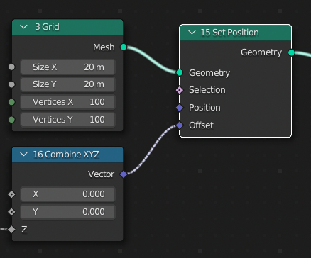
    grid.set_position(offset=(0, 0, z))

The node ‘Set Position’ has 4 input sockets (Geometry, Selection, Position, Offset). In this example, the node is created with the following links:

Geometry : linked with the output socket grid
Selection : no link
Position : no link
Offset : linked ot the output socket of a node ‘Combine XYZ’

This is illustrated here below:

Domains#

Geometry domains are implemented as properties of the geometry classes:

Mesh:
- verts
- faces
- edges
- corners
Curve
- points
- splines
Points (cloud points)
- points
Instances
- insts

Writing grid.set_position() means that you change the position of the grid. But this is not what is done!. In fact, you change the position of the vertices of the grid.

This is why, it is far more better to write:

grid.verts.position += (0, 0, z)

Domains selection#

Operations on domains use a Selection input socket. This feature is implemented in two different ways:

As argument of the domain property:

# Only one vertex on two will be changed

grid.verts((grid.verts.index % 2).equal(0)).position += (0, 0, z)

Using array index:

# Only the vertices between 5000 and 8000 will be changed
grid.verts[5000:8000].position += (0, 0, z)

Both methods can be combined:

grid.verts((grid.verts.index % 2).equal(0))[5000:8000].position += (0, 0, z)

Output geometry#

To define a geometry as the result of the modifier, simply set the output_geometry property of the tree.

    tree.output_geometry = grid.set_shade_smooth()

    # Or you can use the 'shortcut' og
    tree.og = grid.set_shade_smooth()
    

水波#